Introducing Model Builder in QGIS
Attribution note: This workshop is adapted from Ujaval Gandhi’s tutorial, Automating Complex Workflows using Processing Modeler (QGIS3). The original tutorial, workflow idea, and example imagery are credited to Ujaval Gandhi and the QGIS Tutorials and Tips project.
What You Should Understand
By the end of this workshop, you should understand why QGIS Model Builder is useful and how it helps turn a multi-step GIS workflow into something you can run again with one click.
The key idea is simple: instead of repeating every tool manually, you build a model that connects those tools together in a fixed order.
That matters because:
- Your inputs might change.
- You may want to experiment with a different parameter, such as grid size.
- You may want to rerun the same workflow on updated data without rebuilding every step from scratch.
Why Model Builder Matters
Many GIS workflows are really chains of smaller tasks. One tool creates an intermediate output, the next tool uses that output, and so on.
Model Builder is useful because it lets you:
- Describe the workflow once.
- Reuse the workflow later.
- Share the workflow with someone else.
- Run the same process on many inputs as a batch job.
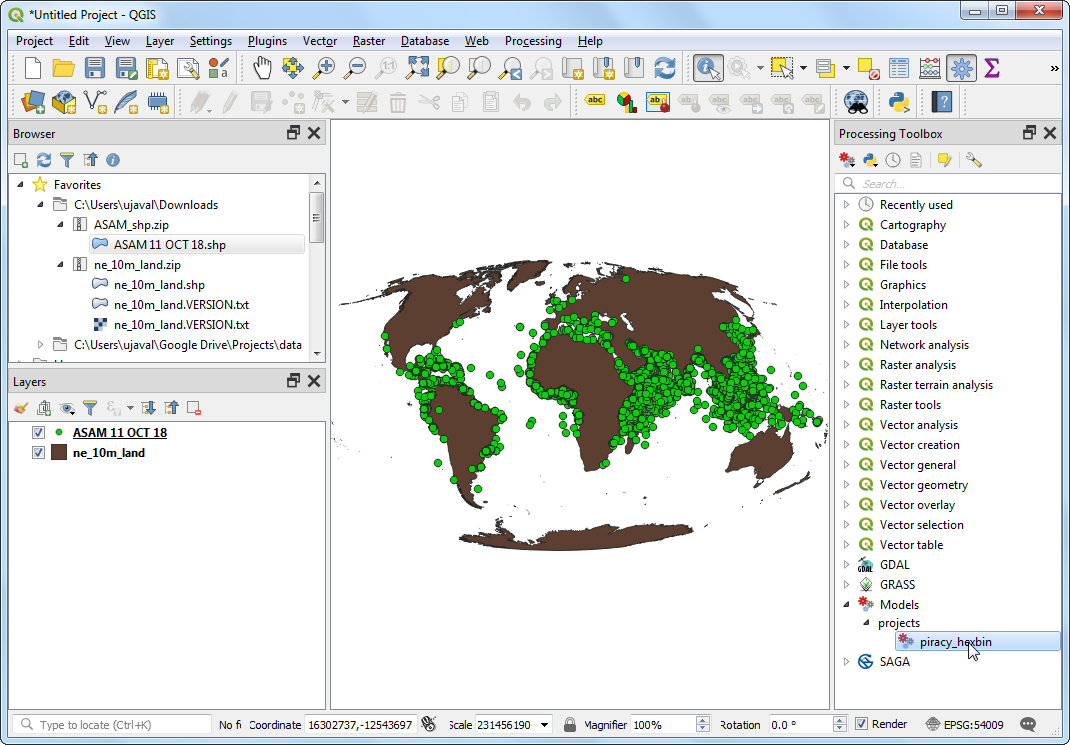
In this exercise, we will build a model that turns the ASAM_events point layer into a density-style map by placing a hexagonal grid over the data and counting how many ASAM_events points fall inside each polygon.
Example Data
This tutorial uses two public datasets:
- The
ASAM_eventspoint layer of maritime piracy incidents from the National Geospatial-Intelligence Agency’s Maritime Safety Information portal. - The
ne_10m_landpolygon layer from Natural Earth.
You can download the same source data directly from the original tutorial page if you want to follow the identical example. For the course version, the important part is not the topic itself but the workflow:
- Start with
ASAM_events. - Reproject
ne_10m_landto match the project. - Create a grid.
- Keep only the grid cells that intersect
ASAM_events. - Count the
ASAM_eventspoints inside each cell. - Style the result.
Getting Ready
If you want to follow the original example exactly, download the source files used in the QGIS tutorial:
These are the same data files used in the original tutorial by Ujaval Gandhi. Save them in a dedicated folder so you can find them easily in the QGIS Browser panel.
Concept Notes
Concept Note: A model is a reusable workflow, not just a one-time map. Once you connect the inputs and algorithms, you can rerun the same logic with different data or different settings.
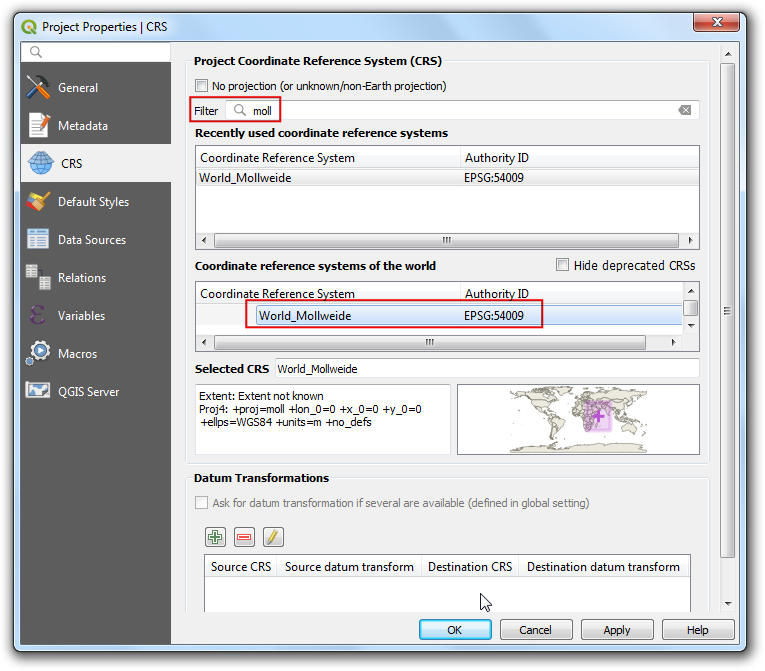
Concept Note: The project CRS matters because some tools need measurements in the units of the project. In this tutorial, the equal-area projection helps the grid cells cover comparable area.
The Workflow We Will Build
Here is the workflow in plain language:
- Accept the
ASAM_eventspoint layer as an input. - Accept the
ne_10m_landpolygon layer as a base layer. - Accept a numeric input for grid size.
- Reproject
ne_10m_landto the project CRS. - Create a hexagonal grid over the extent of the reprojected layer.
- Keep only the grid cells that intersect
ASAM_events. - Count the
ASAM_eventspoints in each remaining polygon. - Symbolize the output using graduated colors.
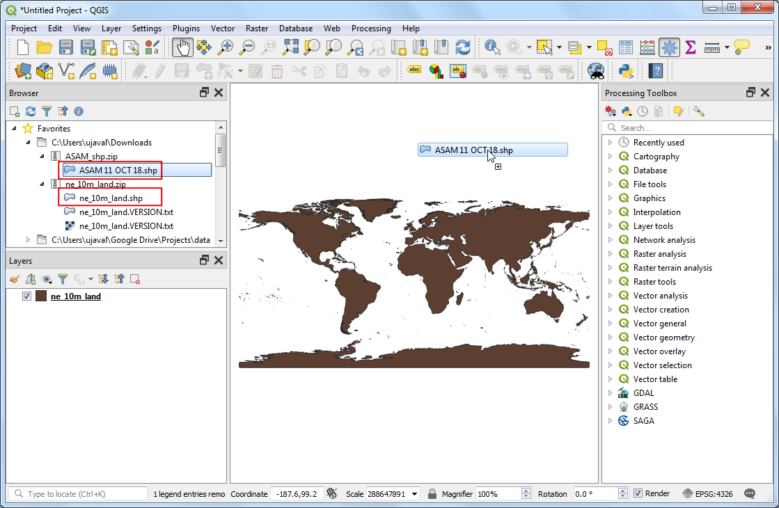
Step 1: Load the Data
Open the two data layers in QGIS:
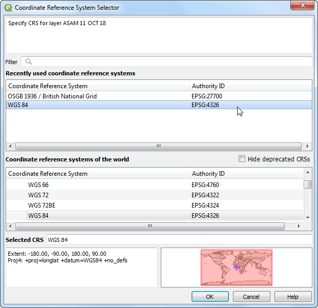
The ASAM_events layer in the original tutorial does not include projection information, so QGIS asks you to define the CRS. Use WGS 84 for the ASAM_events data.
Step 2: Open the Processing Modeler
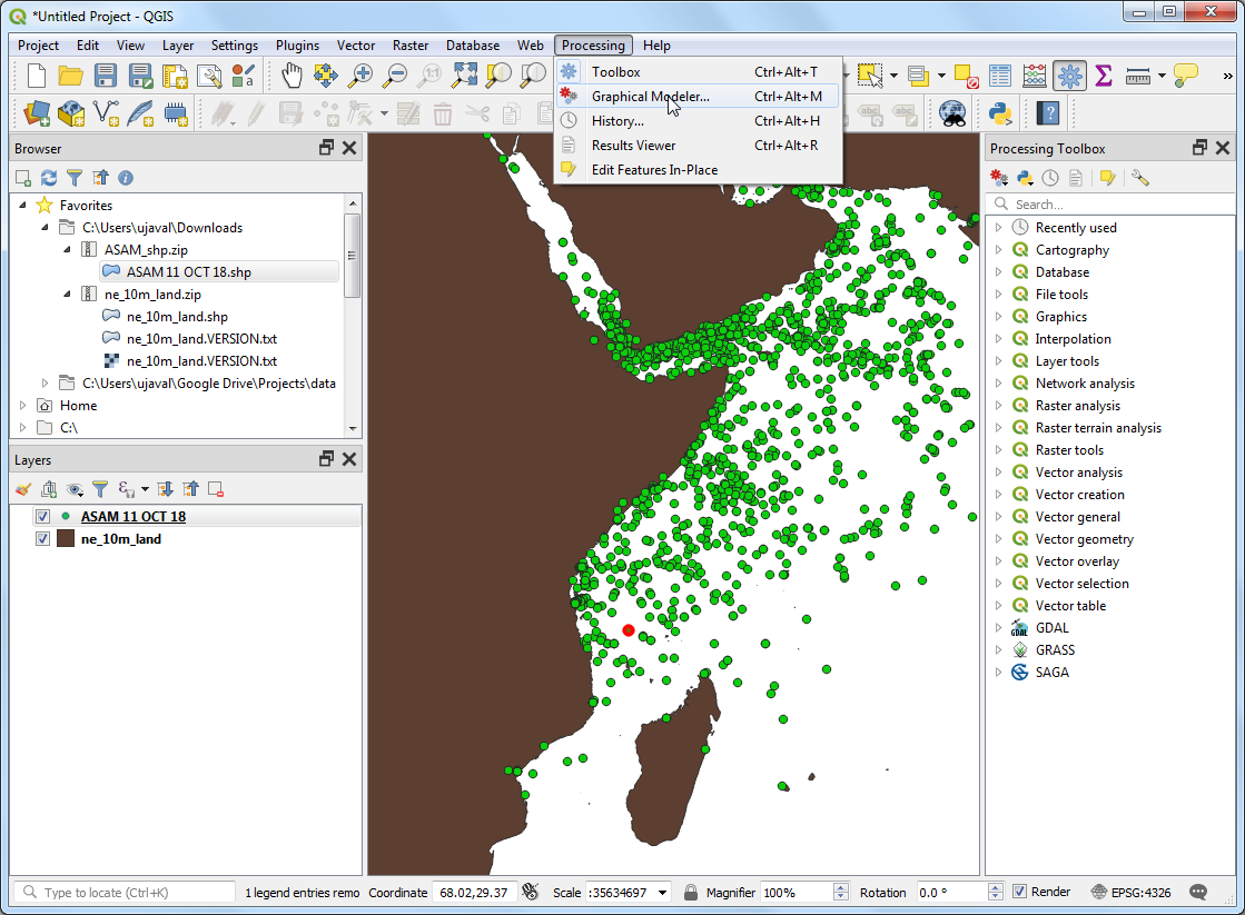
Once the layers are loaded, open the Model Builder from the Processing menu.
In QGIS, go to:
Processing > Graphical Modeler
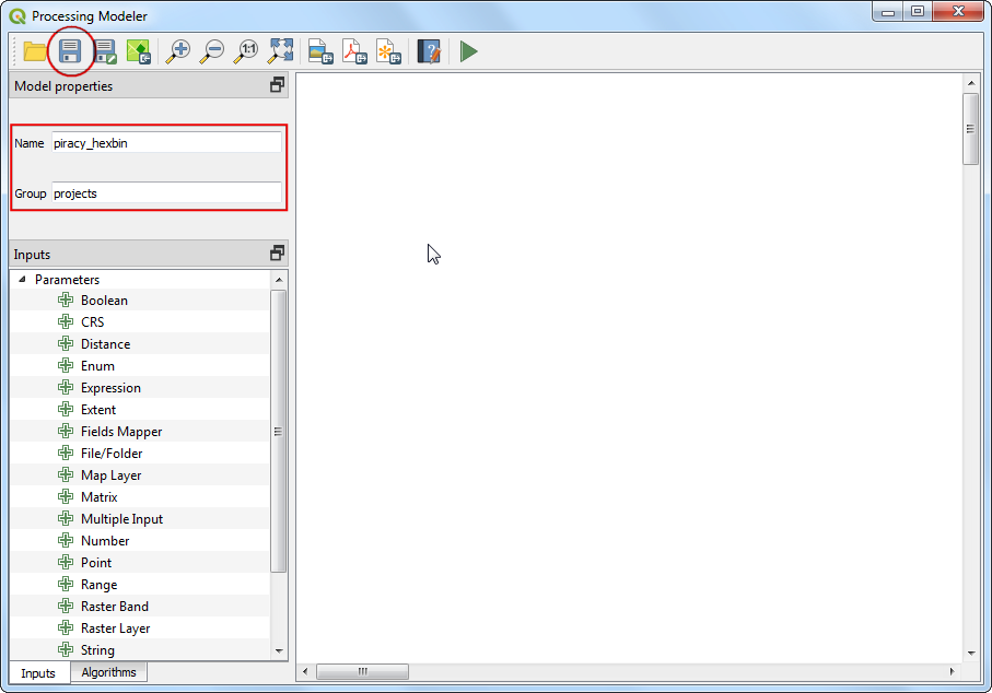
When the Modeler window opens, give the model a name and save it. In the original tutorial, the model is called piracy hexbin.
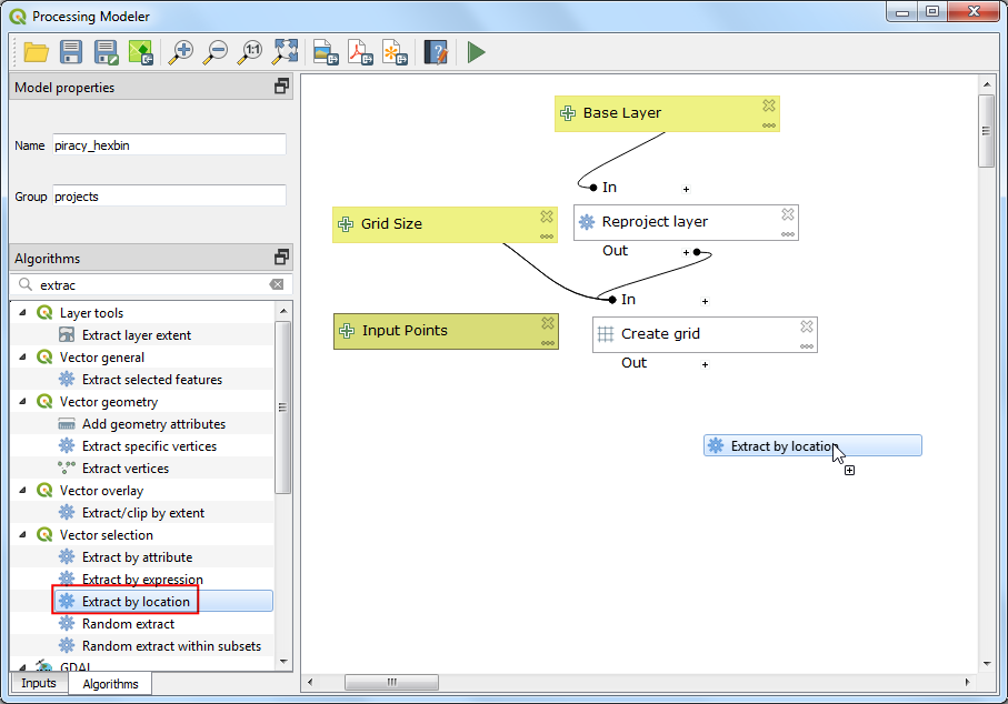
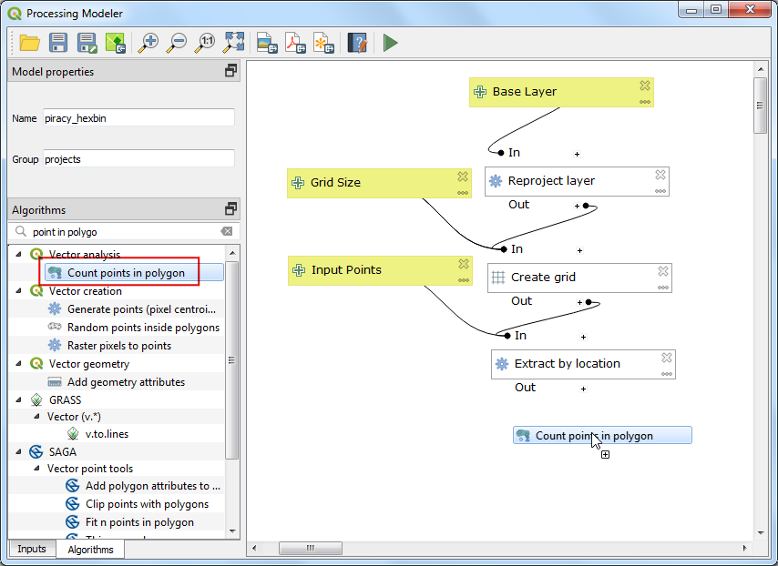
Step 3: Add the Model Inputs
Every model starts with inputs. Inputs are the pieces of information a user can change when the model runs.
For this workflow, we need three inputs:
Add those inputs to the canvas.
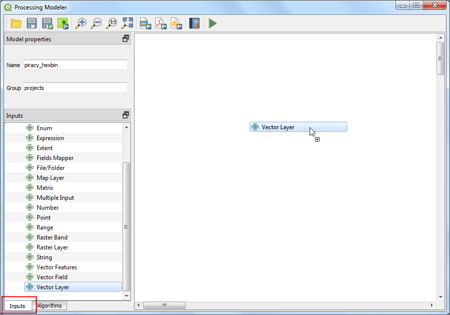
In the original workflow, the point input is named Input Points and is connected to ASAM_events. The polygon input is named Base Layer and is connected to ne_10m_land. The number input is named Grid Size.
Step 4: Reproject the Base Layer
The next step is to reproject ne_10m_land to the project CRS.
Why do this? Because the grid tool needs to work in the units of the project CRS, and a global equal-area projection gives us a better basis for comparing grid cells.
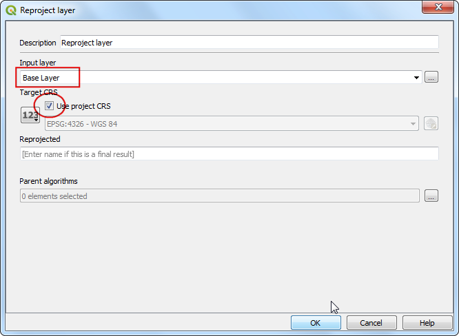
Add the Reproject layer algorithm and connect it to the ne_10m_land base layer input.
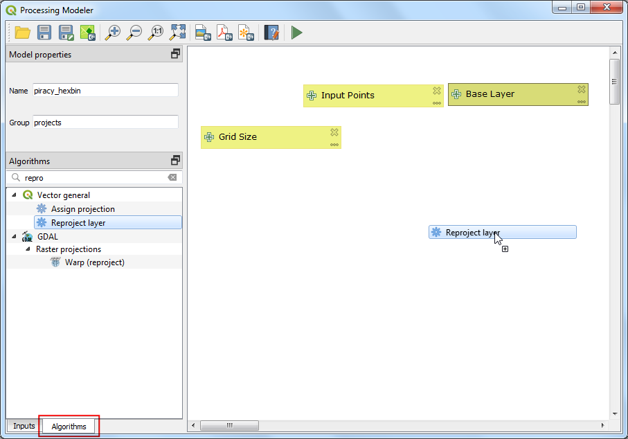
When you configure the algorithm, use ne_10m_land as the input and tell QGIS to use the project CRS as the target CRS.
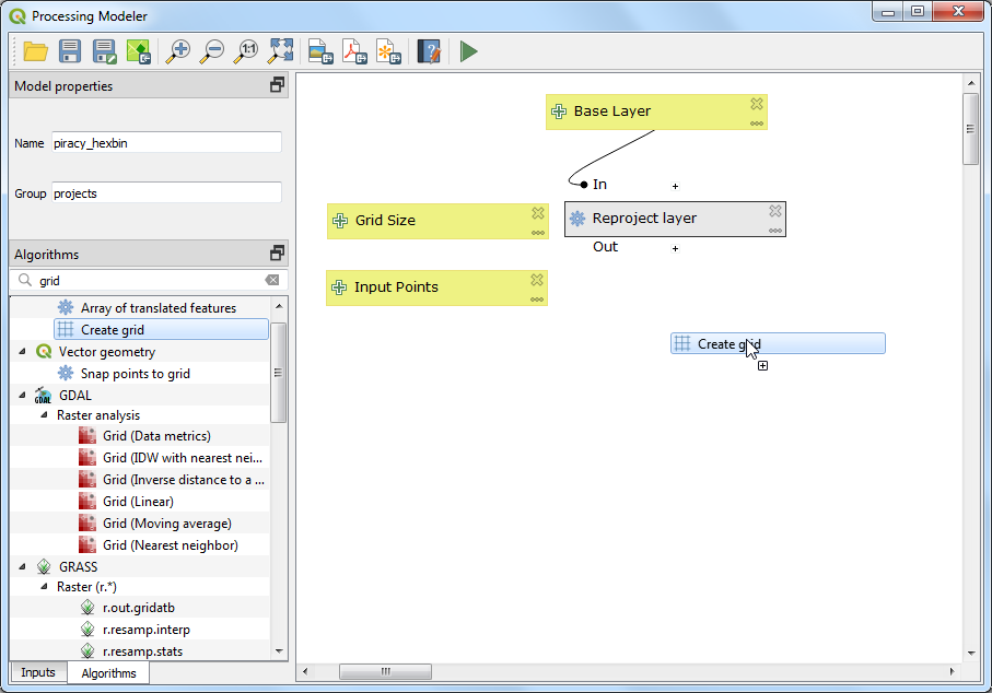
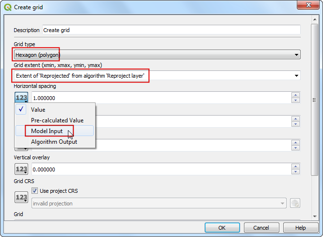
Step 5: Create a Hexagonal Grid
Now add the grid step.
In the original tutorial, the grid is hexagonal. That shape is useful because it creates a regular tessellation without favoring horizontal or vertical directions the way square cells sometimes do.
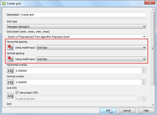
Add the Create grid algorithm and set:
- Grid type:
Hexagon (polygon) - Grid extent: the extent from the reprojected layer
- Horizontal spacing: use the model input for
Grid Size - Vertical spacing: use the same
Grid Sizeinput
Step 6: Keep Only Grid Cells With Data
At this point, the model creates a grid over the full extent of ne_10m_land. Some cells contain ASAM_events, and others do not.
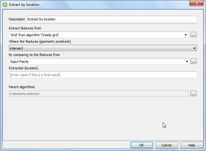
To keep only the useful cells, add Extract by location.
Set it up so the grid cells are extracted where they intersect ASAM_events.
Step 7: Count the Points in Each Polygon
Now we can summarize the ASAM_events points in the cells that remain.
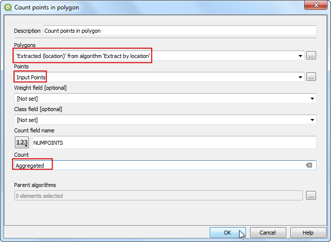
Add Count points in polygon and connect:
- The extracted grid cells as the polygons.
- The
ASAM_eventslayer as the points.
The output will contain a point-count field for each grid cell.
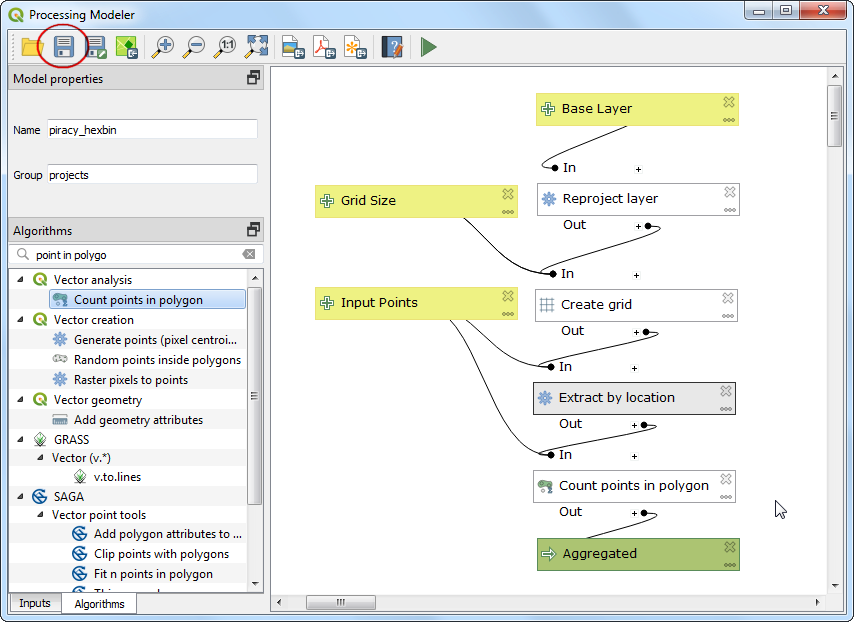
Step 8: Save the Model
Your model is now complete.
Save it so QGIS can reuse it from the Processing Toolbox.
Step 9: Run the Model
Switch back to the main QGIS window.
Before running the model, set the project CRS to a global equal-area projection. The original tutorial uses Mollweide, which works well here because it preserves area better for this kind of summary map.
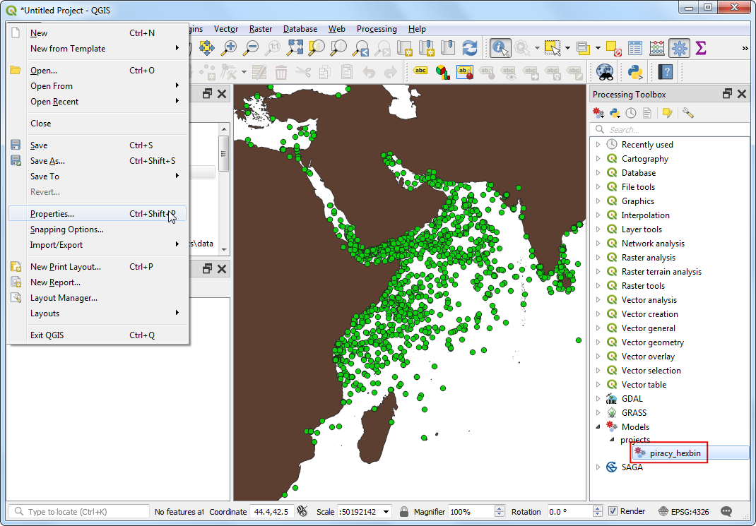
Choose the Mollweide projection in the CRS tab.
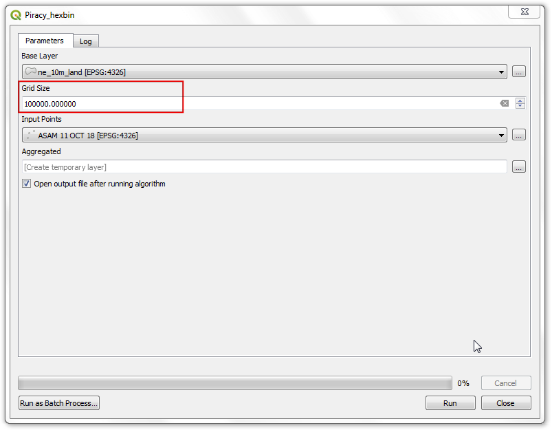
Then open the model from the Processing Toolbox and run it.
Use a grid size that makes sense for the CRS units. In the original example, the grid size is set to 100000 meters.
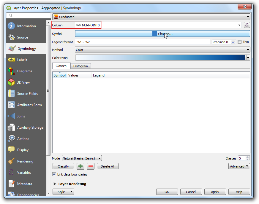
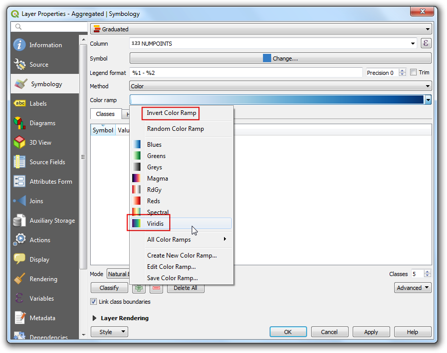
Step 10: Style the Result
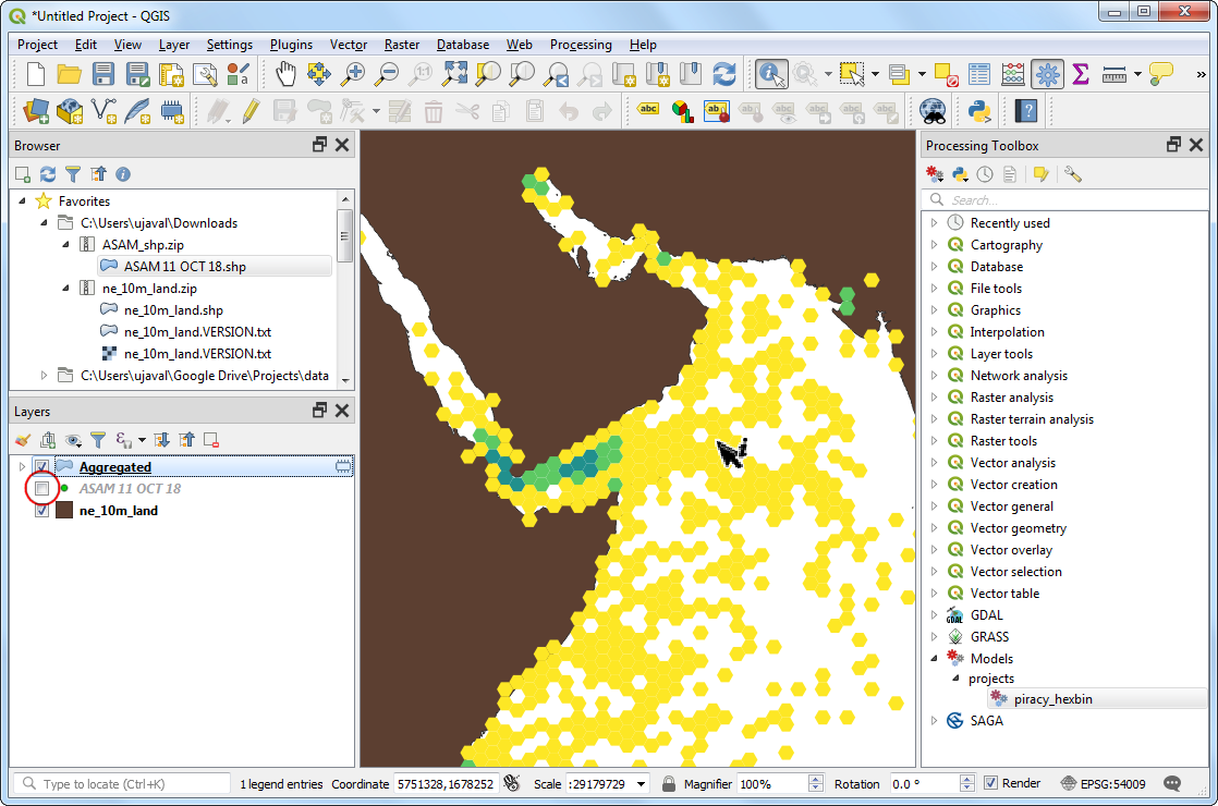
The output layer contains a count field that shows how many ASAM_events points fell into each grid cell.
To make the map easier to read:
- Open the layer properties.
- Switch to Symbology.
- Use
Graduatedstyling. - Choose the count field as the column.
- Use a color ramp such as
Viridis. - Use a classification method such as
Natural Breaks (Jenks).
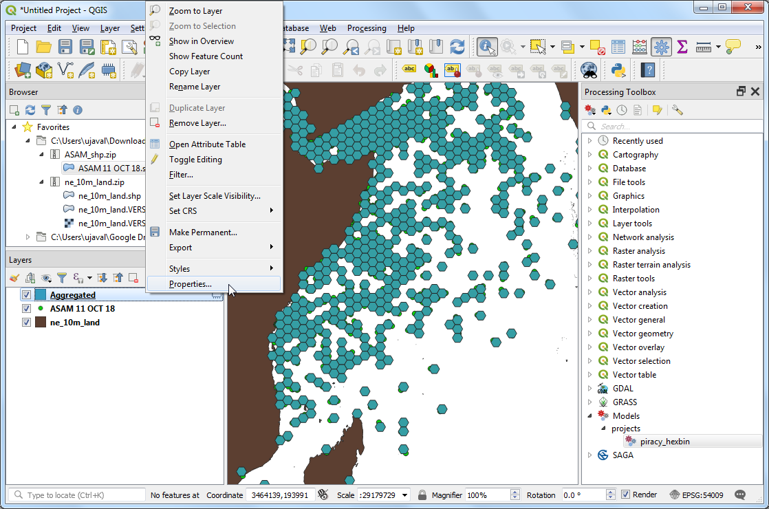
When you turn off the original ASAM_events point layer, you should be able to see the density pattern much more clearly.
What This Teaches
This exercise is not just about one specific map.
It teaches a bigger GIS habit:
- Break a complicated workflow into repeatable pieces.
- Keep the inputs flexible.
- Reuse the model when the data change.
- Use cartography to make the output easier to interpret.