Suitability Modeling in QGIS

Attribution note: This optional workshop is adapted from Ujaval Gandhi’s tutorial, Multi Criteria Overlay Analysis (QGIS3). The workflow, source data organization, and many of the tutorial screenshots are credited to Ujaval Gandhi and the QGIS Tutorials and Tips project.

What You Should Understand

This workshop shows how to answer a common GIS question: where are the places that are most suitable if we combine several criteria at once?

The important idea is that suitability analysis is not just about making one layer look good. It is about translating a set of geographic rules into a repeatable workflow that can be measured, combined, weighted, and mapped.

By the end of the exercise, you should understand:

1. Why raster workflows are often better than vector overlays for multi-criteria suitability analysis.
2. Why NoData handling matters when converting vector layers to raster.
3. How to reclassify continuous raster values into suitability scores.
4. How to combine multiple criteria with the Raster Calculator.

Concept Note: Vector overlay tools are excellent for yes/no questions, such as whether a parcel intersects a buffer. Raster suitability analysis is better when you want to rank places and combine more than a few criteria.

Getting Ready

Download the tutorial data package from the original QGIS tutorial:

• assam.gpkg

The GeoPackage contains the five layers used in the analysis:

1. boundary
2. roads
3. protected_regions
4. water_polygons
5. water_polylines

Concept Note: The boundary layer is important twice. First, it gives us a shared extent for the raster outputs. Later, it helps us mask out pixels outside the study area so the final map is easier to read.

Overview of the Task

In the original tutorial, the goal is to find places in Assam, India that are:

• close to roads,
• away from water bodies, and
• not inside protected regions.

That is a classic suitability question. Each criterion contributes a score, and the final raster combines those scores into one map of relative suitability.

Step 1: Load the Data

Open assam.gpkg in the QGIS Browser and drag the five layers into the map canvas.

You should see boundary, roads, protected_regions, water_polygons, and water_polylines in the Layers panel.

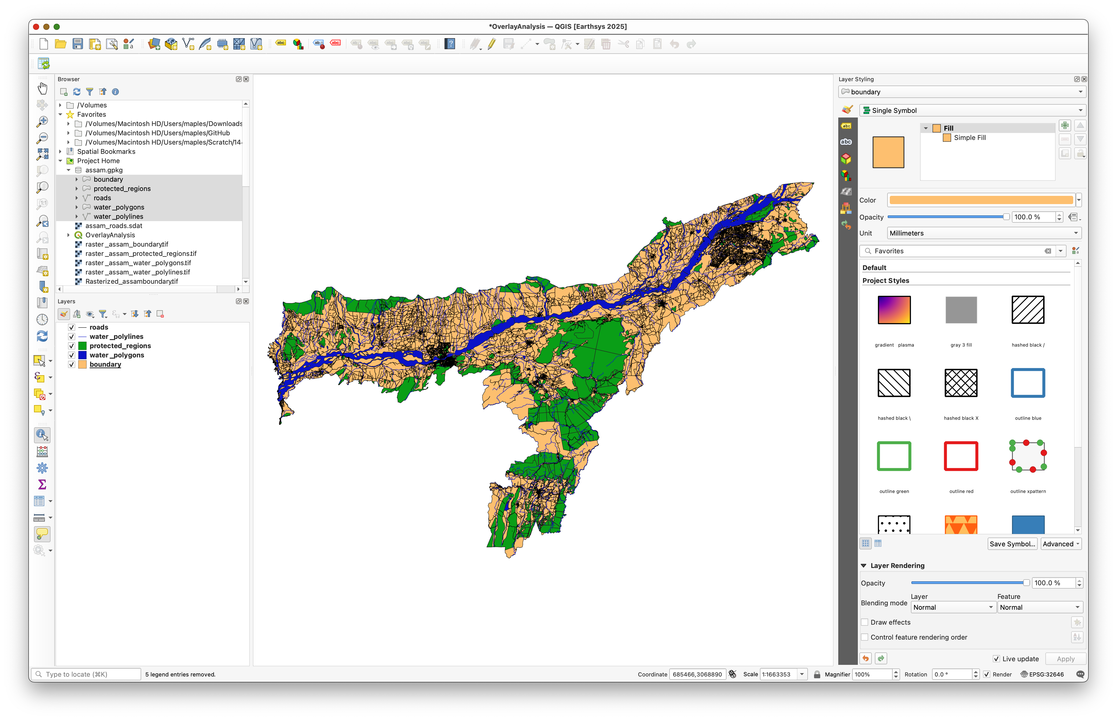
The layers are already clipped to Assam, which keeps the example manageable and lets us focus on the overlay logic.

Step 2: Rasterize the boundary Layer

Before we rasterize the thematic layers, we need a raster mask for boundary.

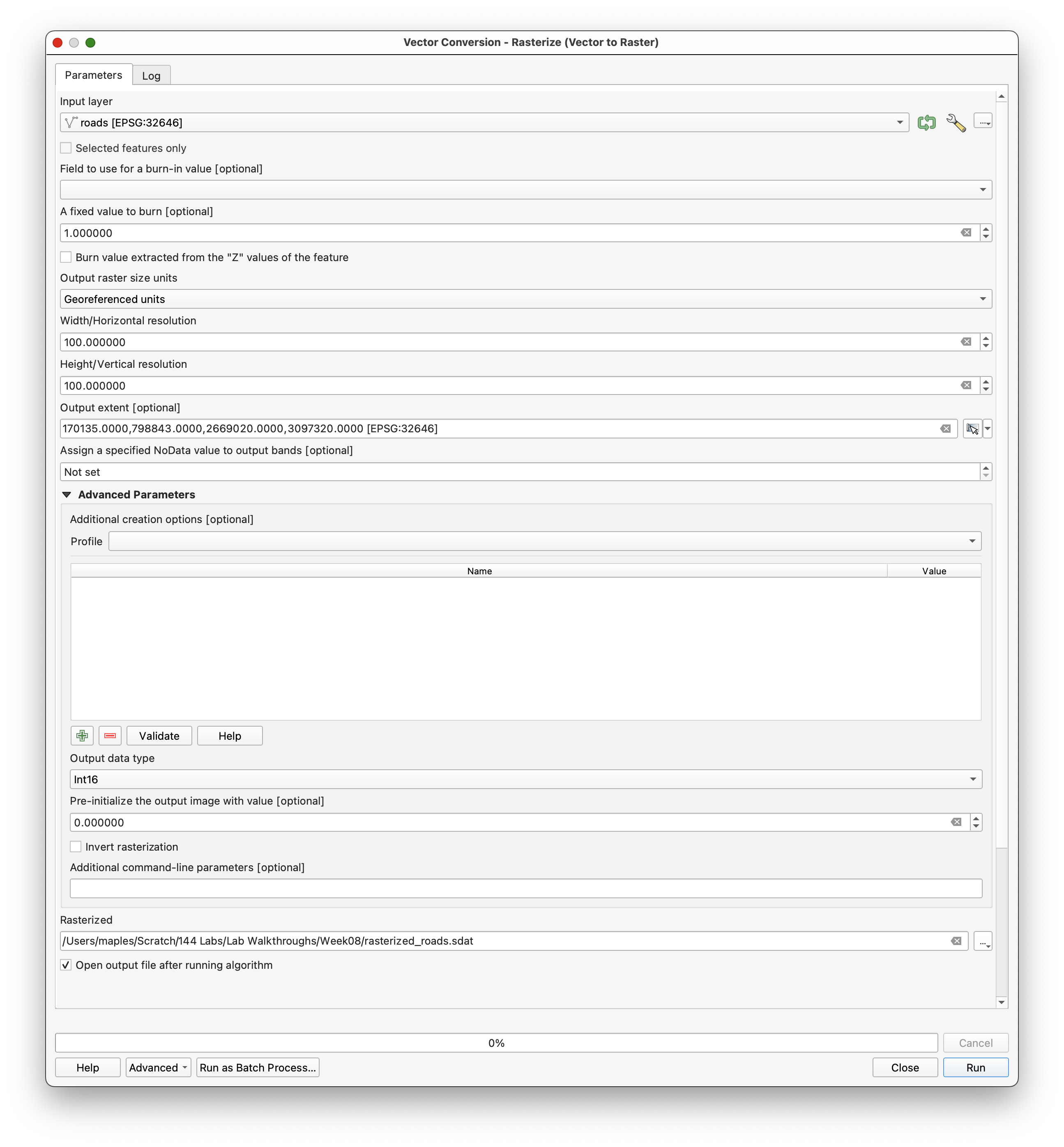
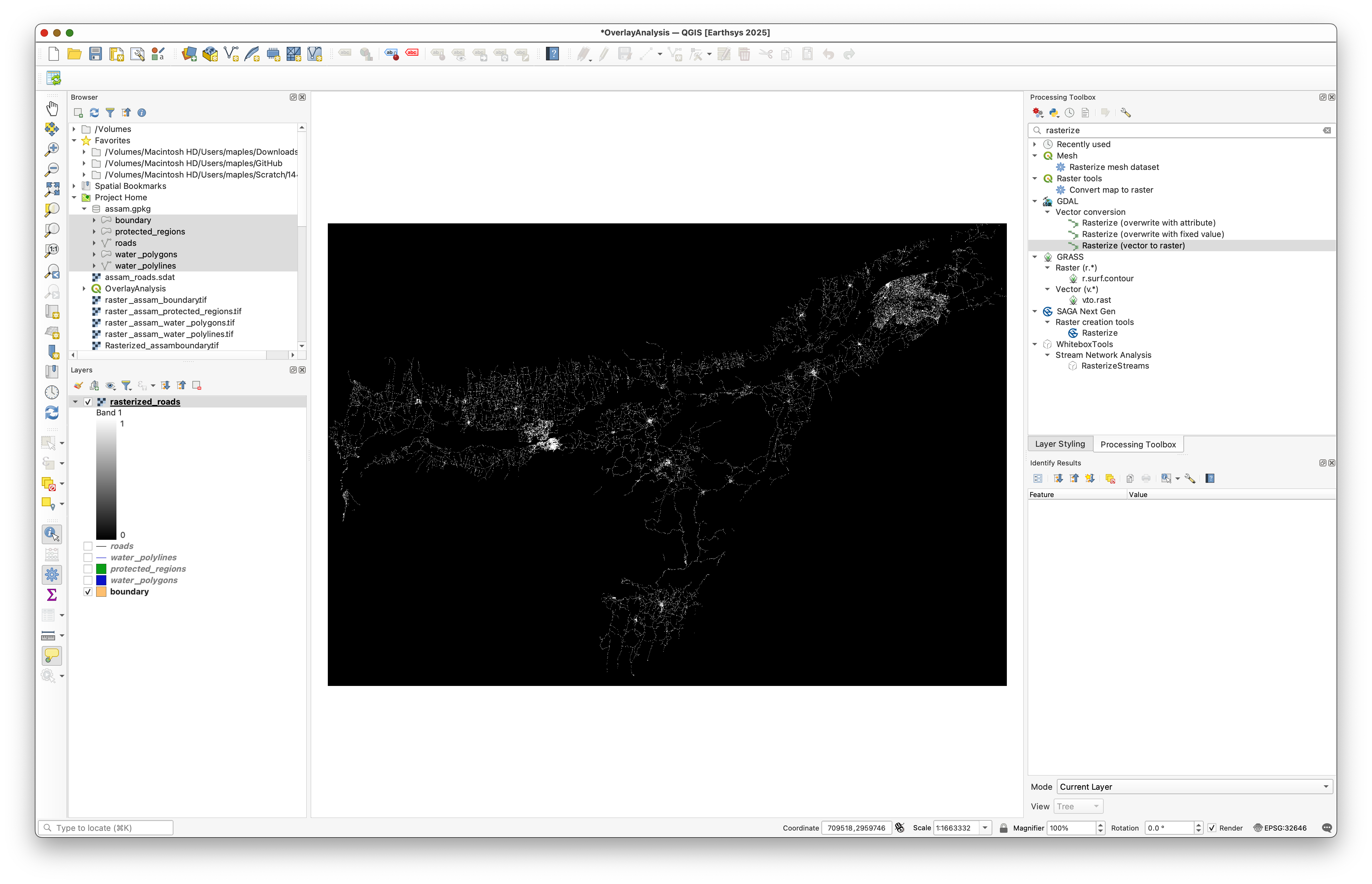
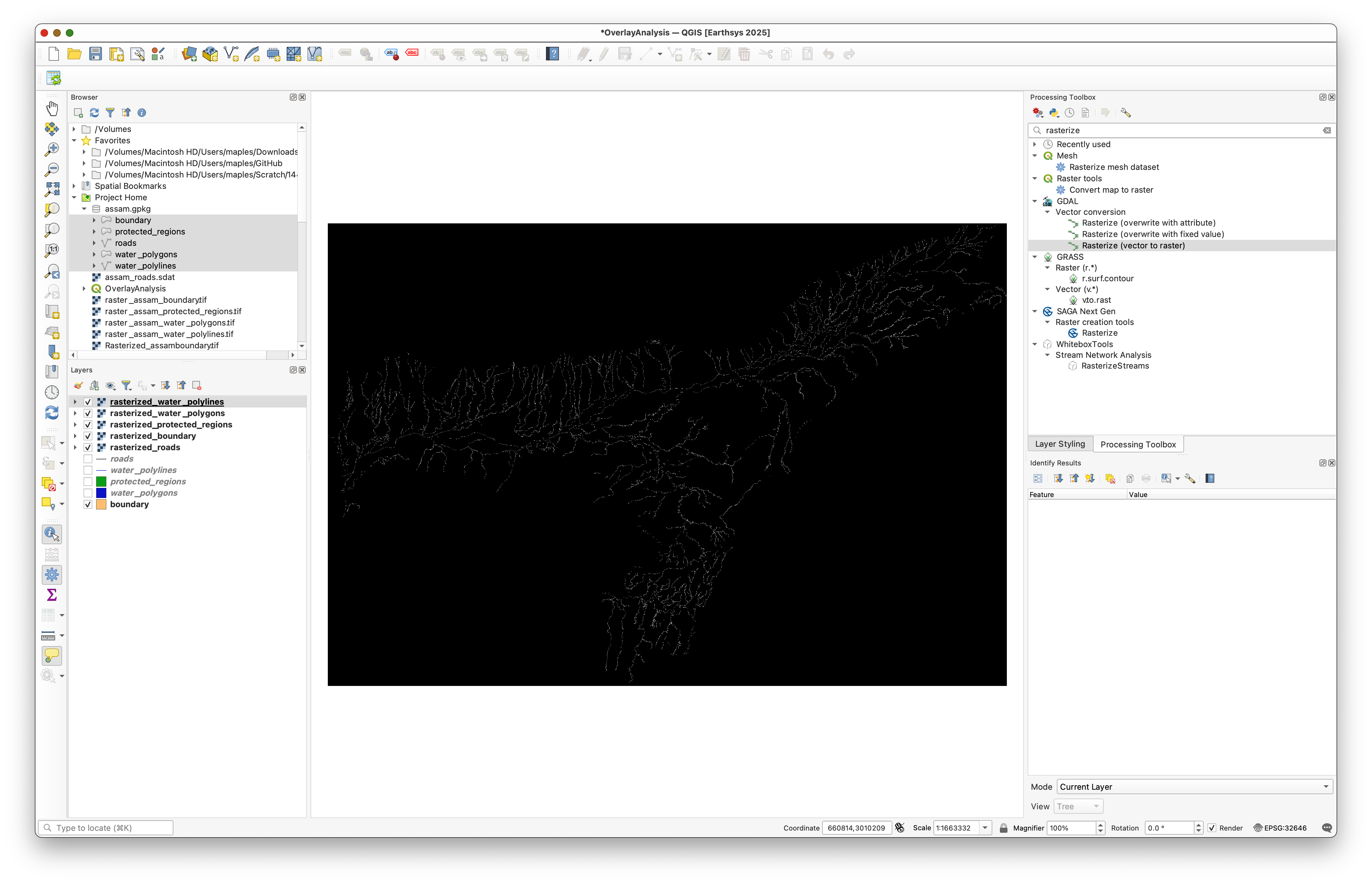
Use the Processing Toolbox and search for Rasterize (vector to raster).

Set the tool up so:

1. boundary is the input layer.
2. The burn value is 1.
3. The raster size units are Geoferenced units.
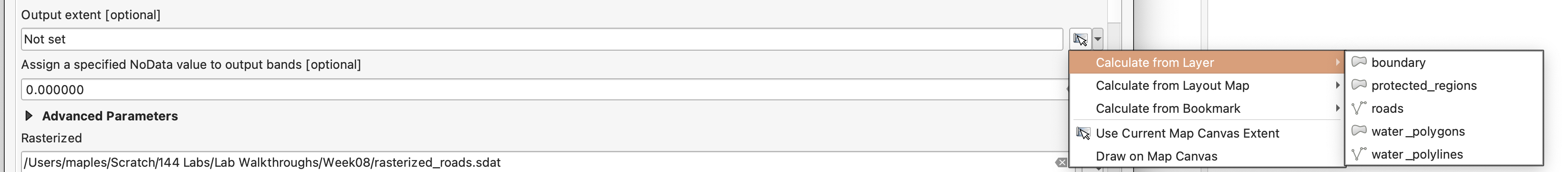
4. The resolution is 15 meters by 15 meters.
5. The output extent is calculated from boundary.
6. The output data type is Int16.
7. The output image is pre-initialized with 0.
8. The output file is saved as rasterized_boundary.tif.

Concept Note: The raster resolution controls the level of detail in the output. Smaller pixels capture more detail but make the workflow heavier to run.

Step 3: Rasterize and Fill roads

Now rasterize roads with the same extent and resolution settings.

Use:

1. Input layer: roads
2. Burn value: 1
3. Output size units: Geoferenced units
4. Resolution: 15 meters
5. Output extent: from boundary
6. Output data type: Int16
7. Pre-initialized value: 0
8. Output file: raster_roads.tif

After rasterizing, the roads layer contains NoData where no roads were present. That is a problem for later calculations, because Raster Calculator treats NoData specially.

Use Fill NoData cells to replace NoData with 0, and save the result as raster_roads_filled.tif.

Concept Note: Filling NoData with 0 makes the raster behave like a true presence/absence layer. That is much easier to combine later than a layer full of missing values.

Step 4: Batch Rasterize the Remaining Layers

Rather than repeating the same rasterization and fill steps manually, use Batch Processing for the other thematic layers:

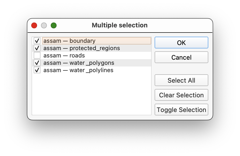
1. protected_regions
2. water_polygons
3. water_polylines

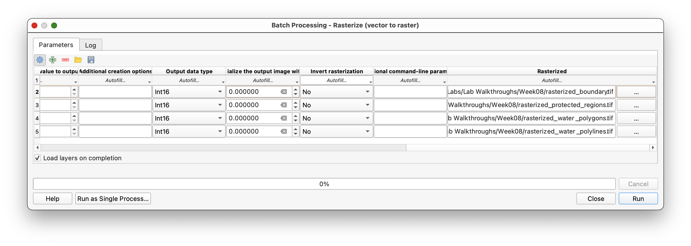
Open Rasterize (vector to raster) and choose Execute as Batch Process.

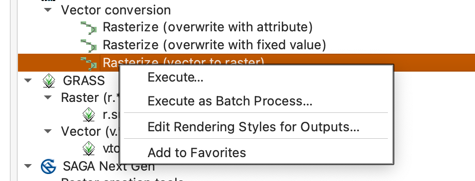
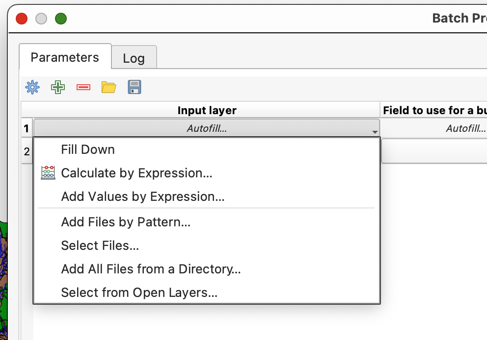
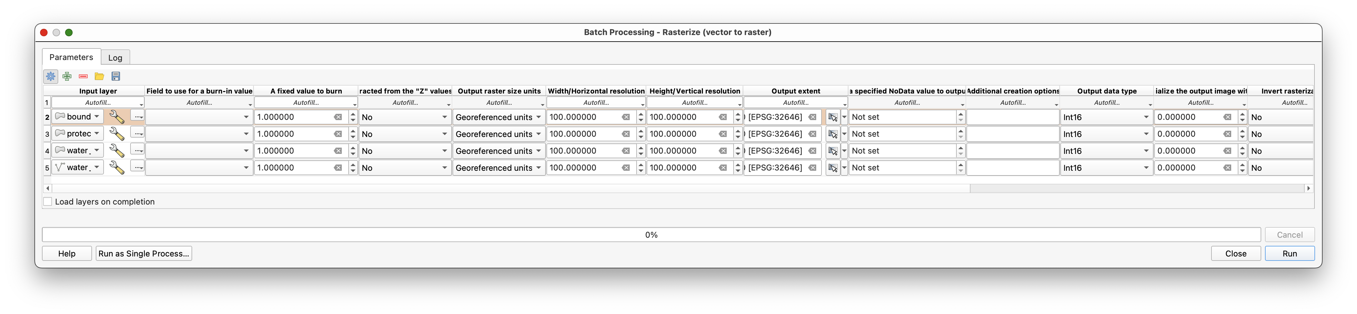
In the batch dialog:

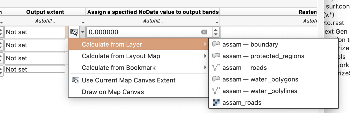
1. Use Select from Open Layers... to fill the input layer column.
2. Use Fill Down to repeat the shared raster settings.
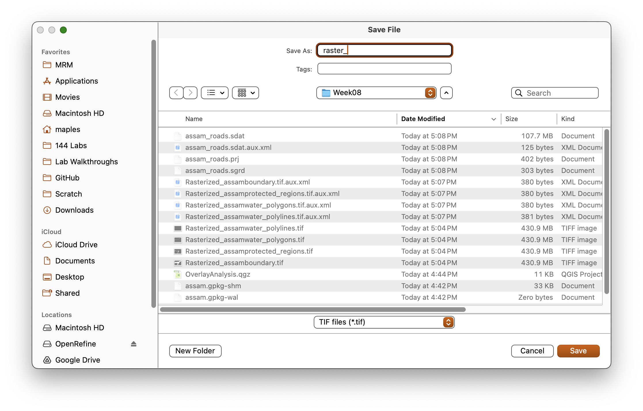
3. Keep the output extent tied to boundary.
4. Set the output file prefix to raster_.
5. Make sure the layers load when the batch finishes.

After rasterization, fill the NoData values for those rasters too, so you end up with:

• raster_protected_regions_filled
• raster_water_polygons_filled
• raster_water_polylines_filled

You should also keep rasterized_boundary and raster_roads_filled in the project.

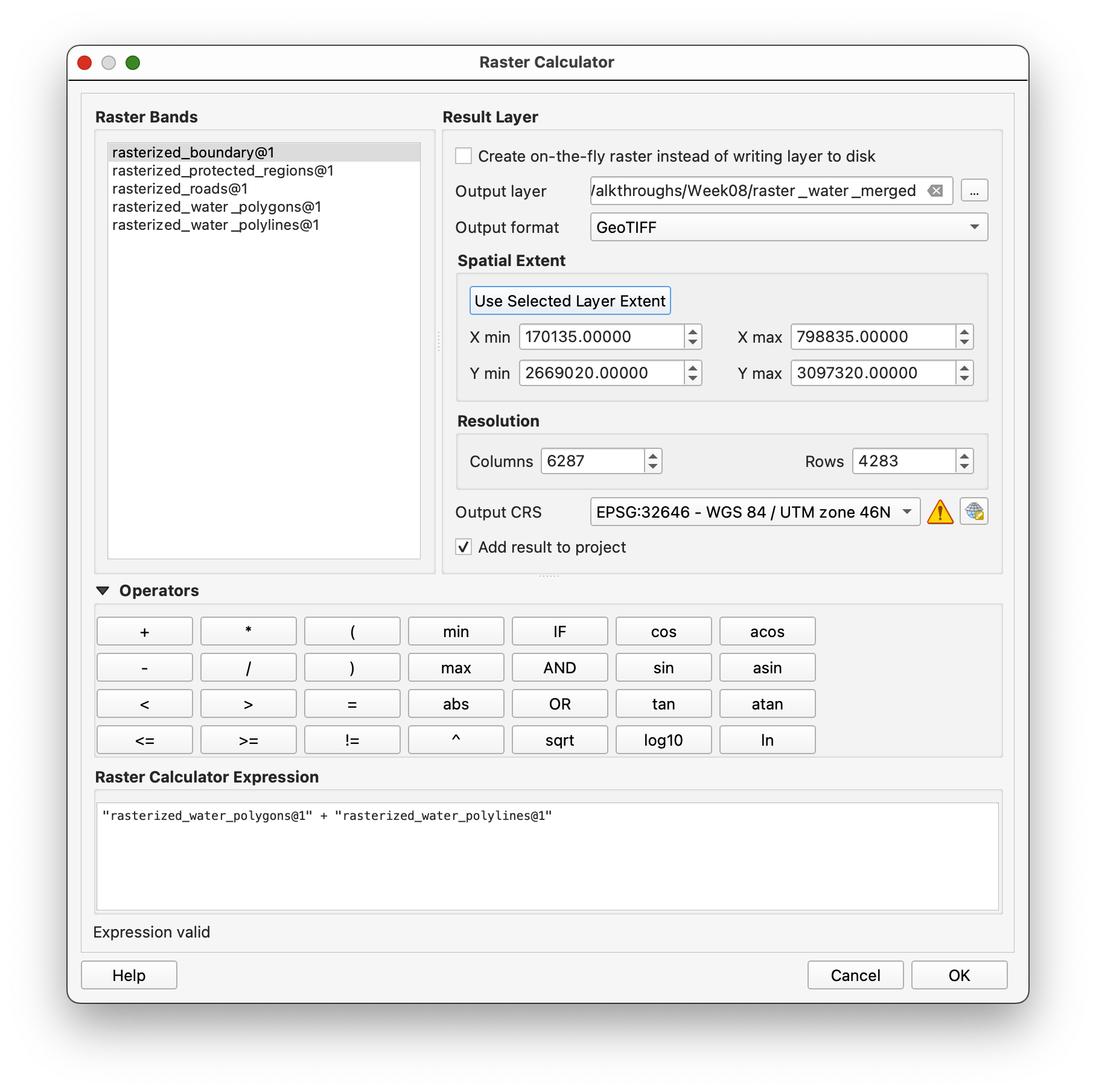
Step 5: Merge the Water Layers

We now have two water layers, one for polygons and one for polylines. Since both represent water, we can combine them into a single layer.

Open Raster calculator and add the two filled water rasters together:

"raster_water_polygons_filled@1" + "raster_water_polylines_filled@1"

Use rasterized_boundary as the reference extent and save the result as raster_water_merged.tif.

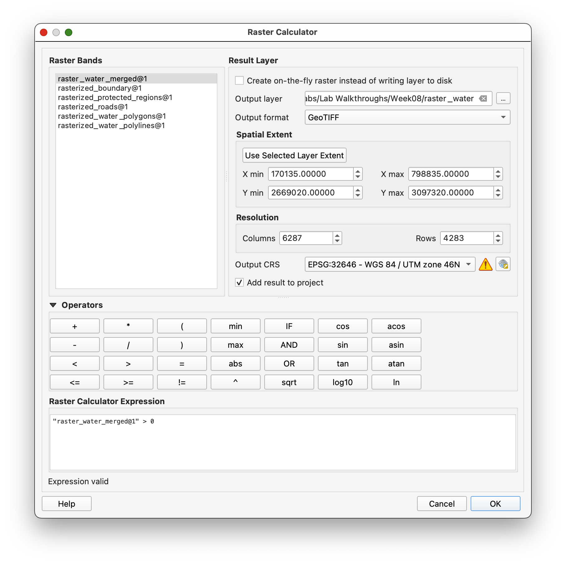
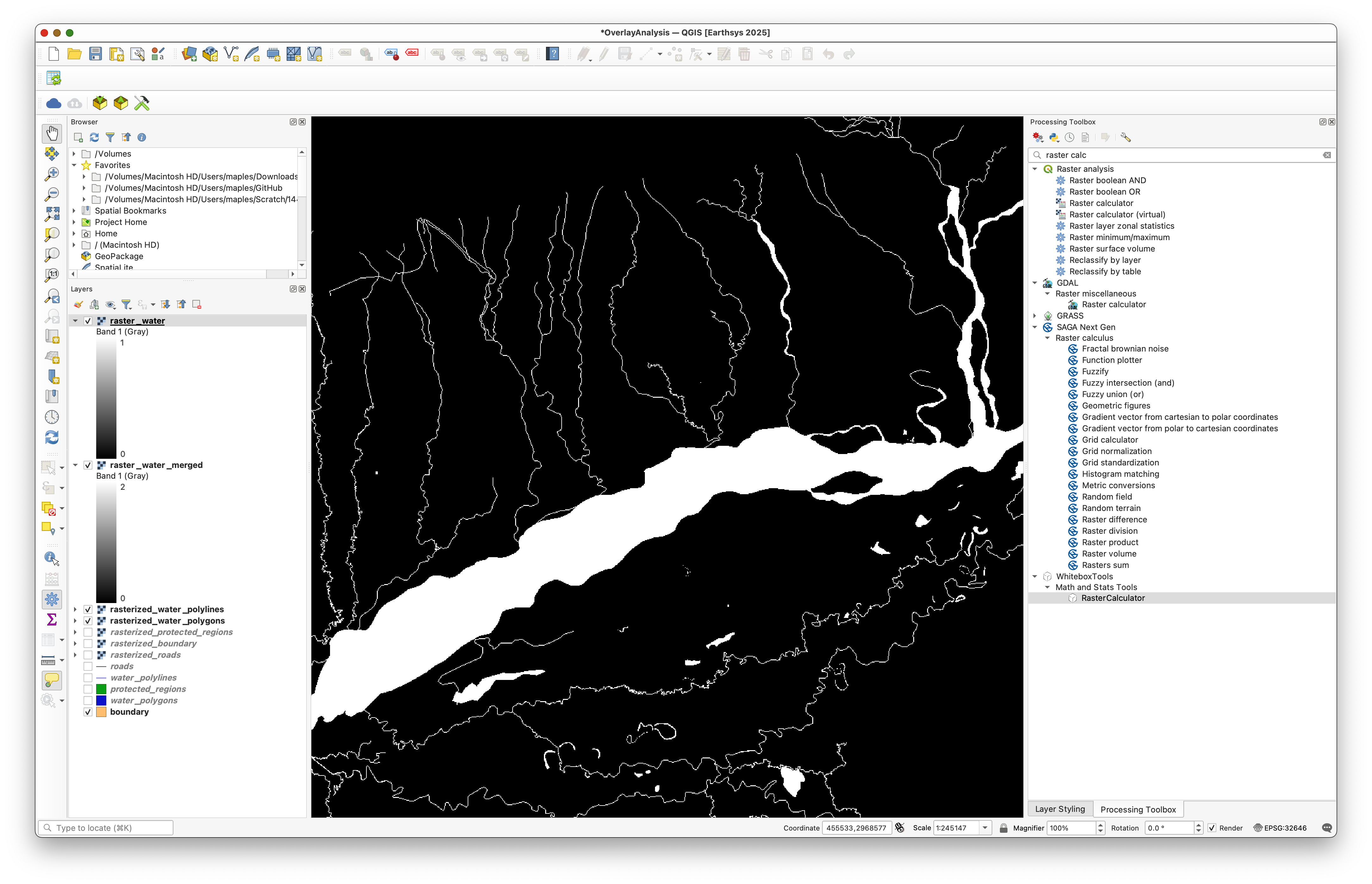
The merged water raster may contain pixels with a value of 2 where polygon and polyline water overlap. That is not what we want for a simple presence/absence mask.

Use Raster calculator again with:

"raster_water_merged@1" > 0

Save the output as raster_water_filled.tif.

Concept Note: Raster Calculator is useful because it lets us turn a messy intermediate raster into a cleaner analysis layer with simple logical rules.

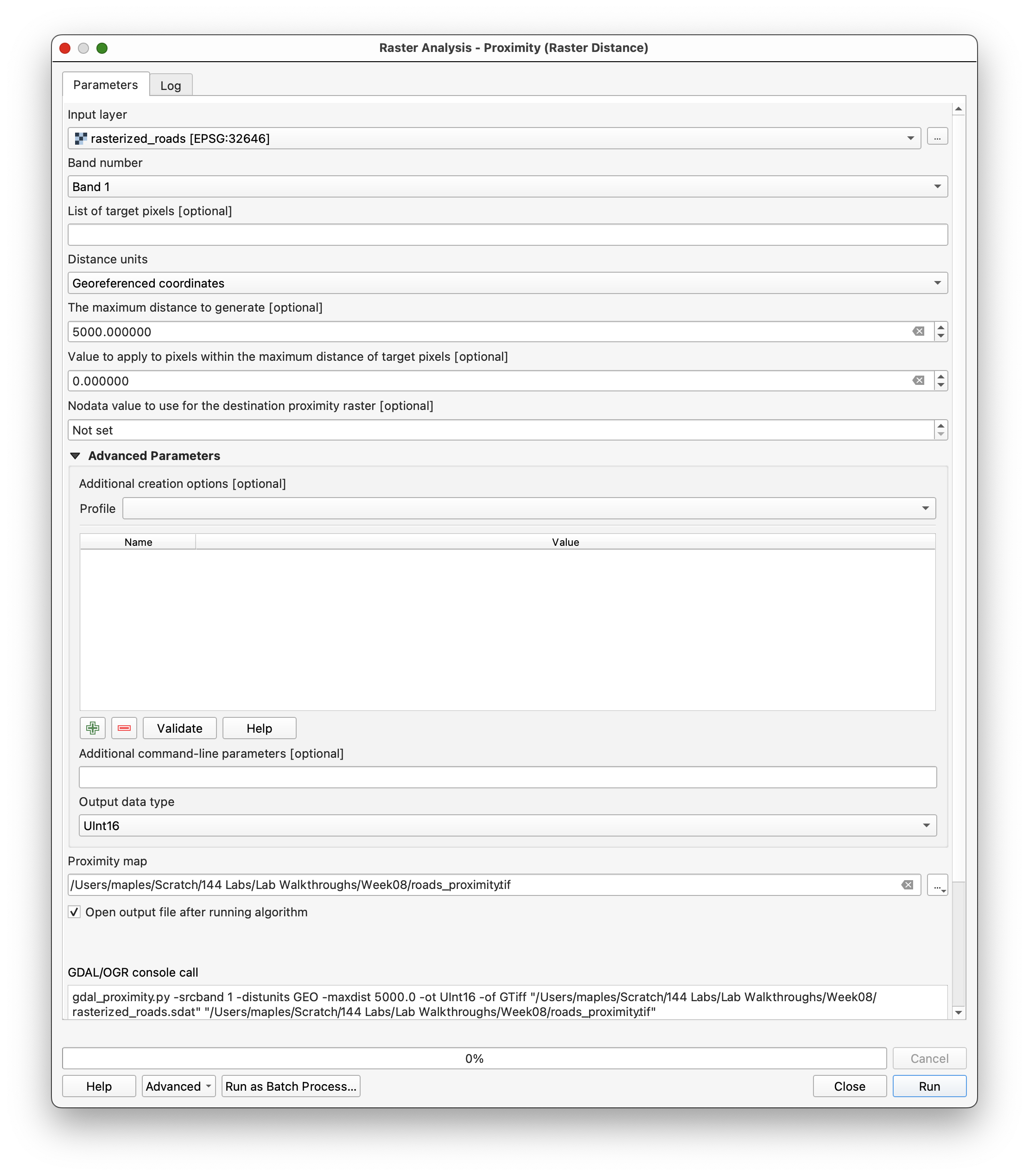
Step 6: Generate Proximity Rasters

Distance to roads and water matters in the suitability model, so we need distance rasters.

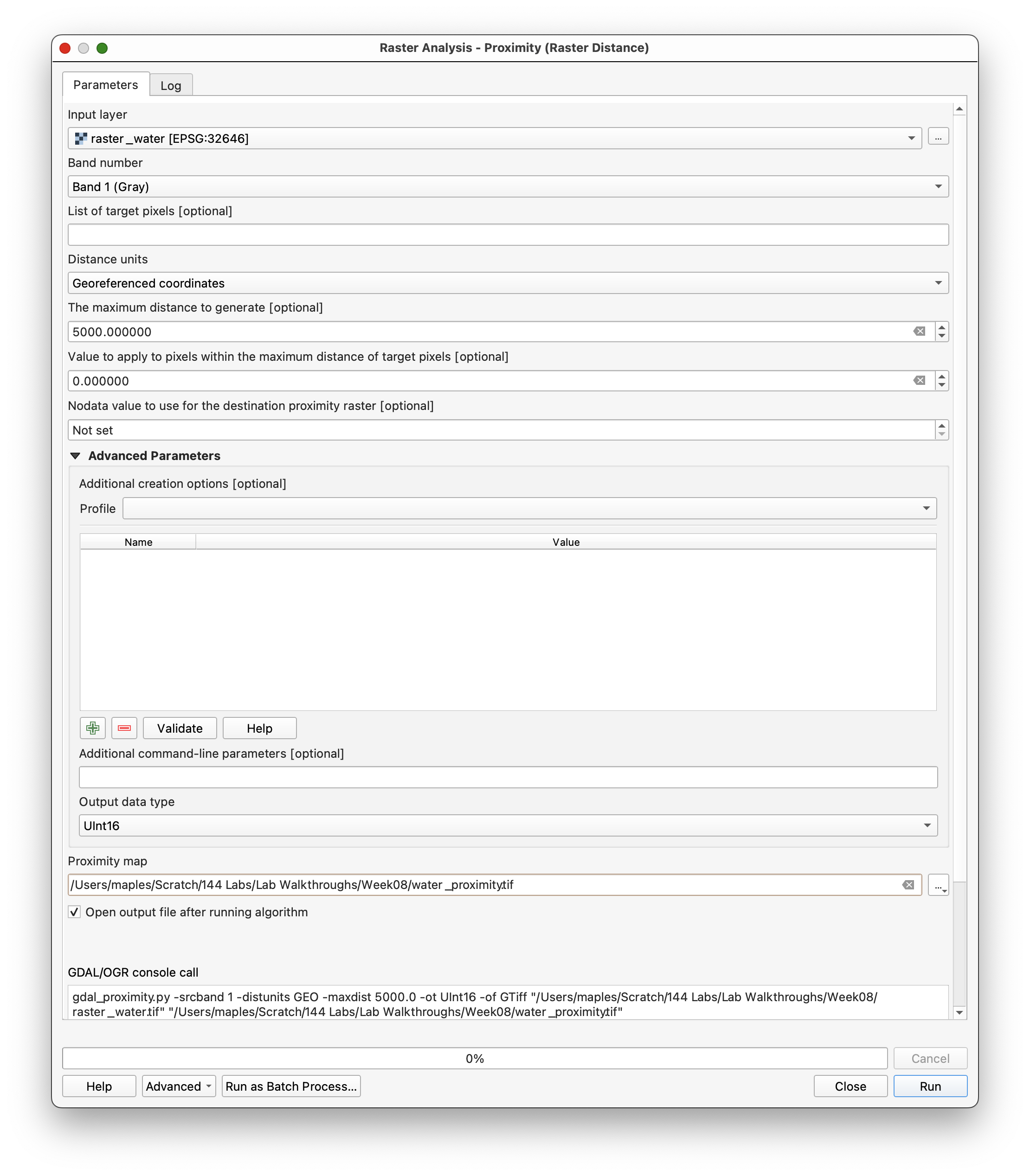
Use Proximity (raster distance) for raster_roads_filled:

1. Input layer: raster_roads_filled
2. Distance units: Georeferenced coordinates
3. Maximum distance: 5000
4. NoData value: 5000
5. Output data type: Int16
6. Output file: roads_proximity.tif

Once the raster is created, adjust the styling so the distance values are easier to read.

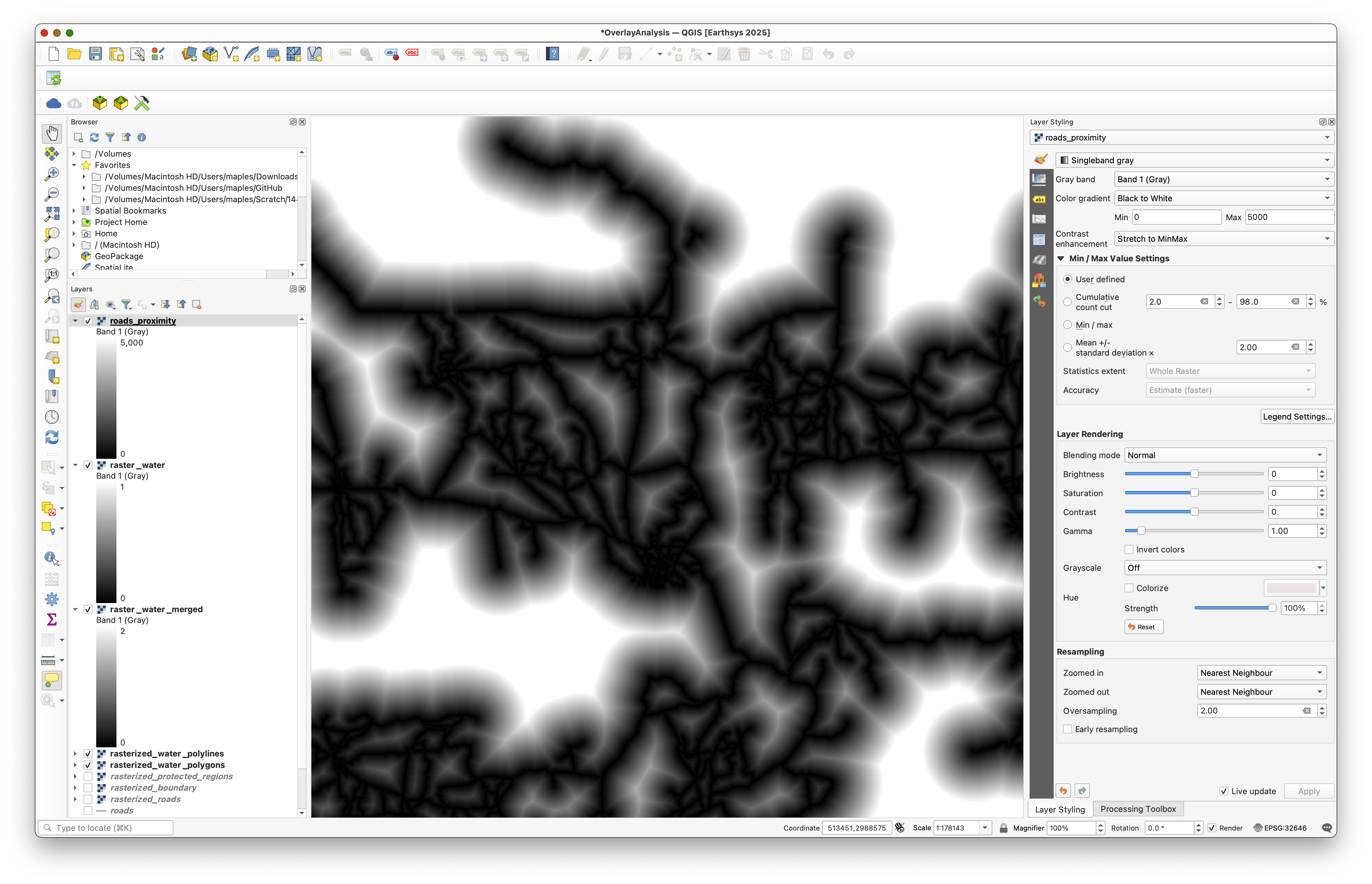
Repeat the same proximity workflow for raster_water_filled and save the result as water_proximity.tif.

Step 7: Reclassify the Distance Rasters

Distance rasters are continuous values, but suitability analysis usually needs simpler categories.

We will convert the road and water proximity rasters into suitability scores.

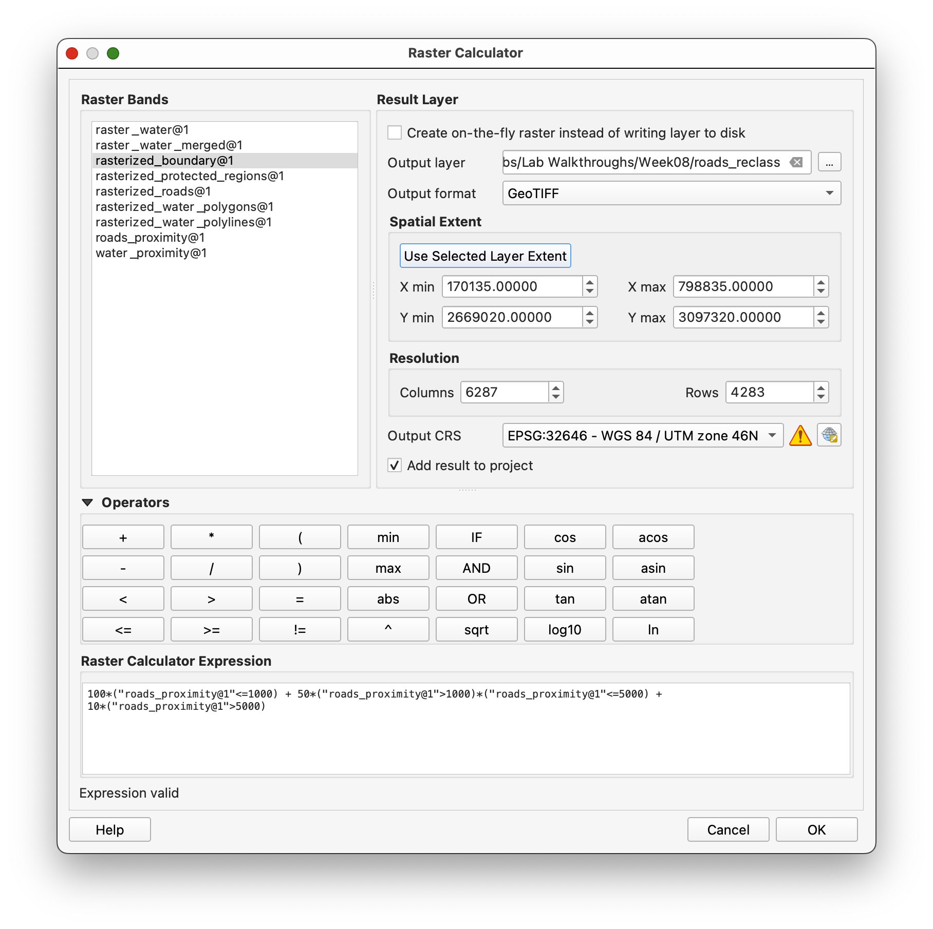
For roads, nearer is better:

• 0-1000 m = 100
• 1000-5000 m = 50
• >5000 m = 10

Use Raster calculator with:

100*("roads_proximity@1"<=1000) + 50*("roads_proximity@1">1000)*("roads_proximity@1"<=5000) + 10*("roads_proximity@1">5000)

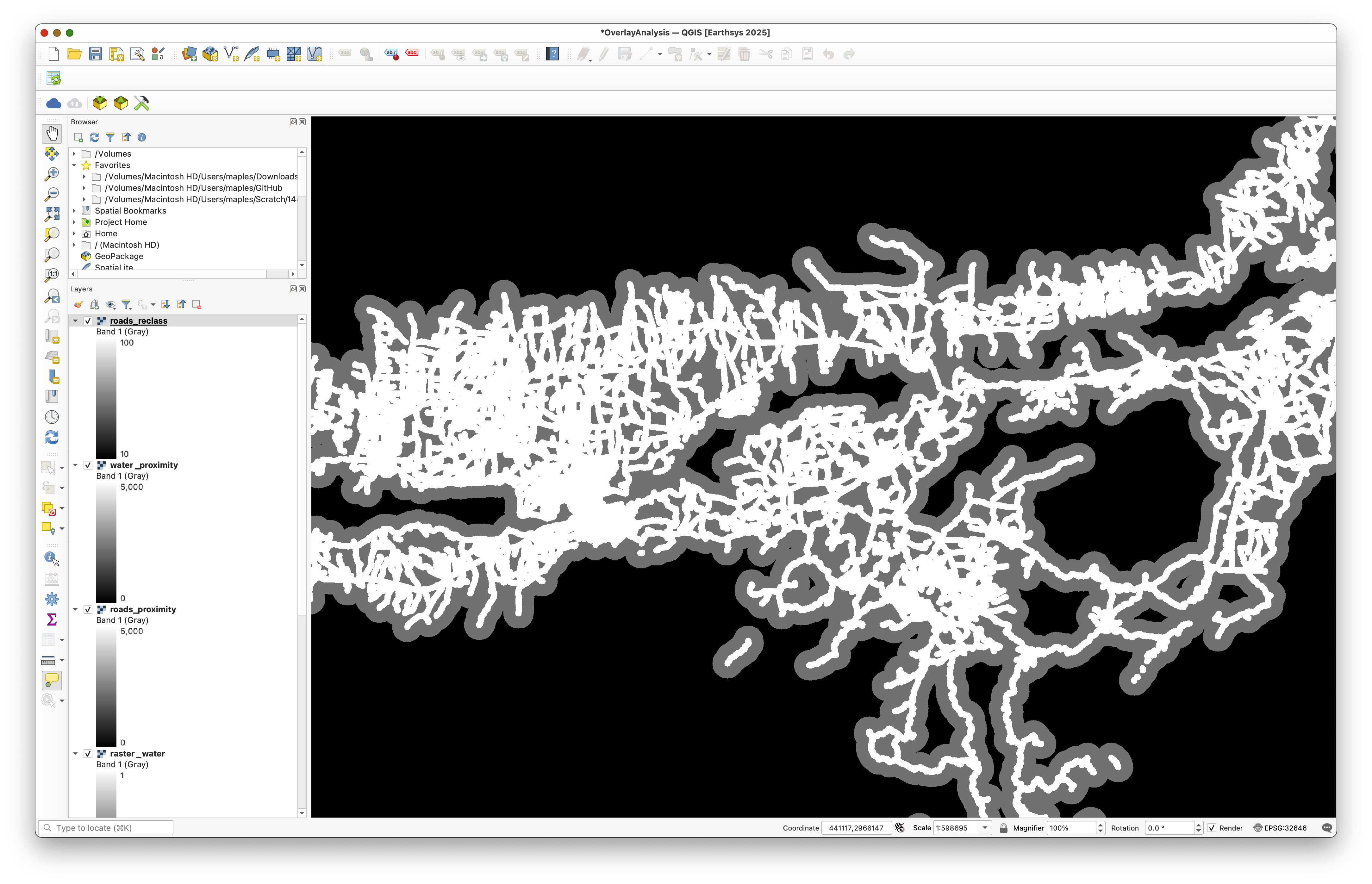
Save the result as roads_reclass.tif.

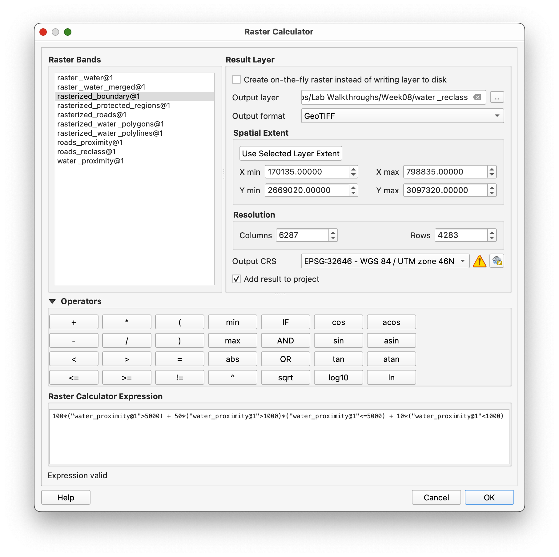
For water, farther is better:

• 0-1000 m = 10
• 1000-5000 m = 50
• >5000 m = 100

Use:

100*("water_proximity@1">5000) + 50*("water_proximity@1">1000)*("water_proximity@1"<=5000) + 10*("water_proximity@1"<1000)

Save the output as water_reclass.tif.

Concept Note: Reclassification turns a continuous measurement into a simple scoring system. That makes it easier to combine several criteria in one formula.

Step 8: Build the Final Suitability Raster

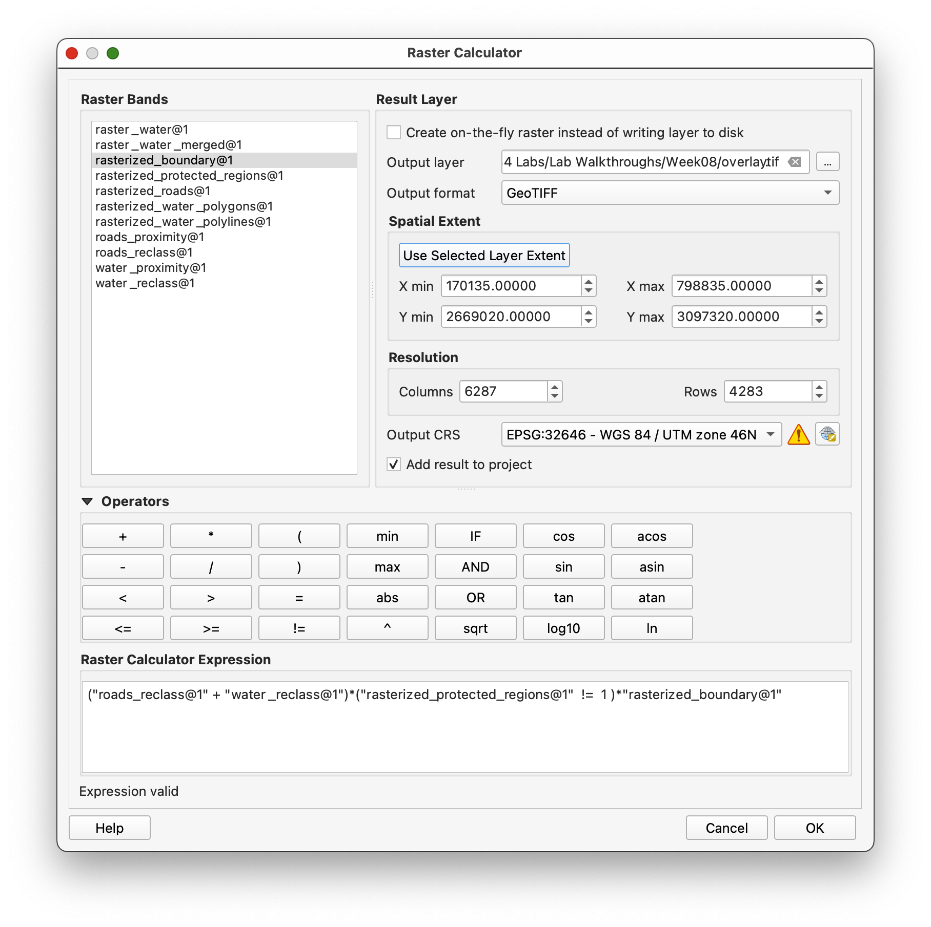
Now combine the reclassified road and water layers, then remove protected regions and keep the result inside the boundary.

Use Raster calculator with this expression:

("roads_reclass@1" + "water_reclass@1")*("raster_protected_regions_filled@1" != 1)*"rasterized_boundary@1"

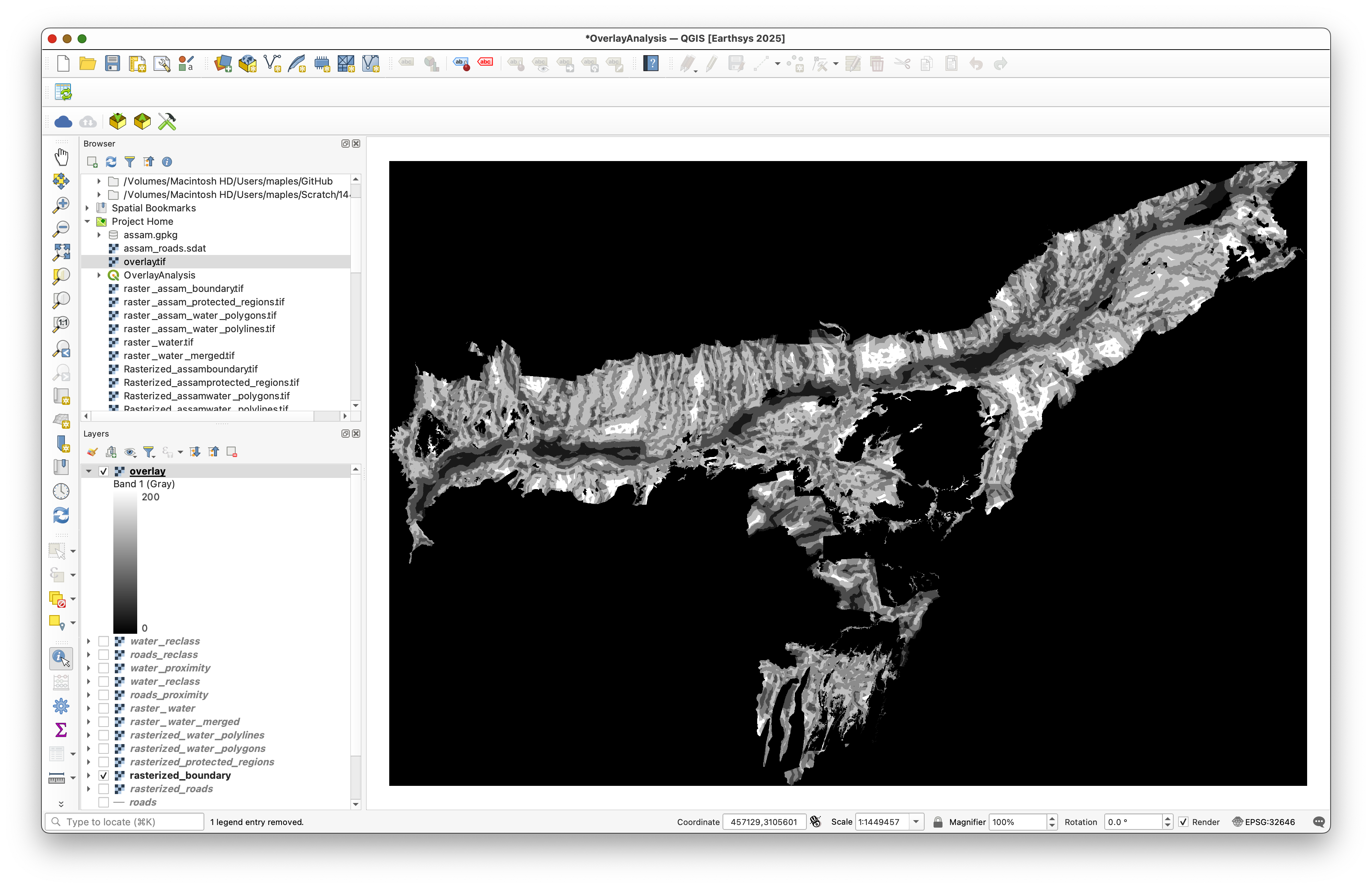
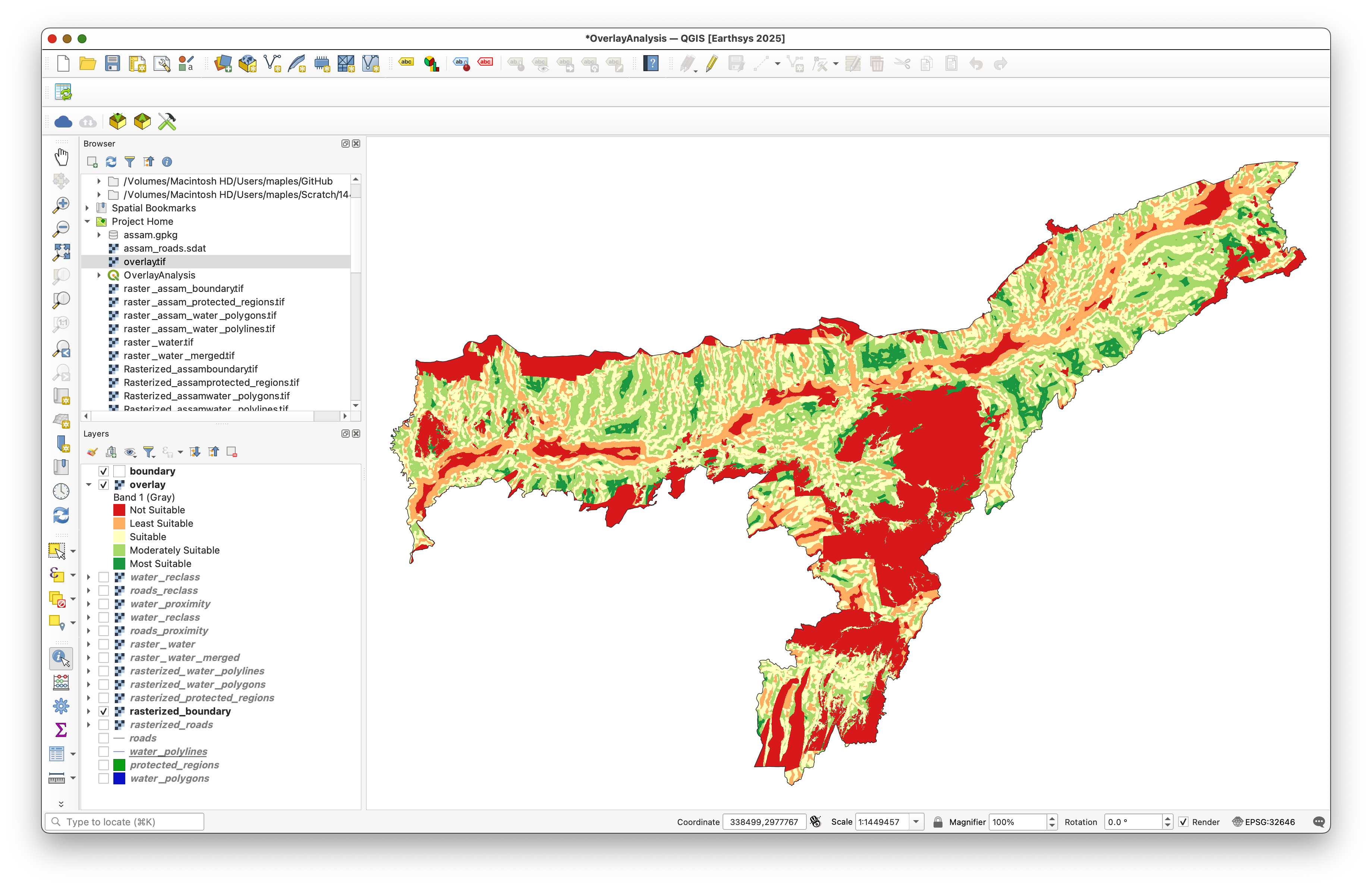
Save the output as overlay.tif.

This is the final suitability map. Higher values mean more suitable areas, and lower values mean less suitable areas.

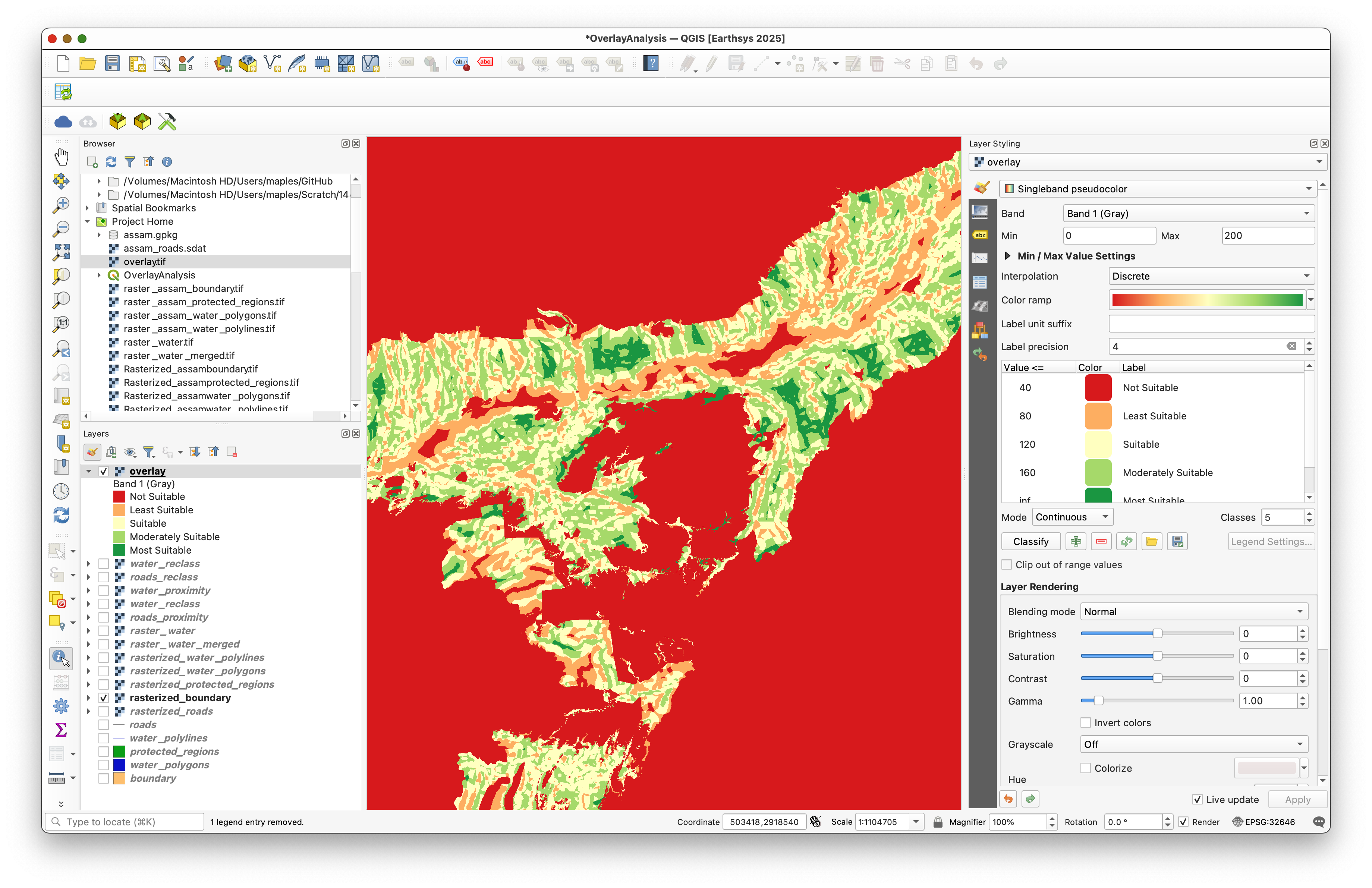
Step 9: Style the Map

Open the layer styling panel for overlay and set:

1. Renderer: Singleband pseudocolor
2. Color ramp: a ramp that clearly separates suitable from unsuitable values
3. Labels: edit the default class labels so the legend is easier to interpret

Step 10: Use an Inverted Polygon Mask for the Layout

To hide pixels outside the study area in a layout, change the boundary layer to use the Inverted Polygons renderer.

This gives the map a clean study-area edge while keeping the final raster visible inside Assam.

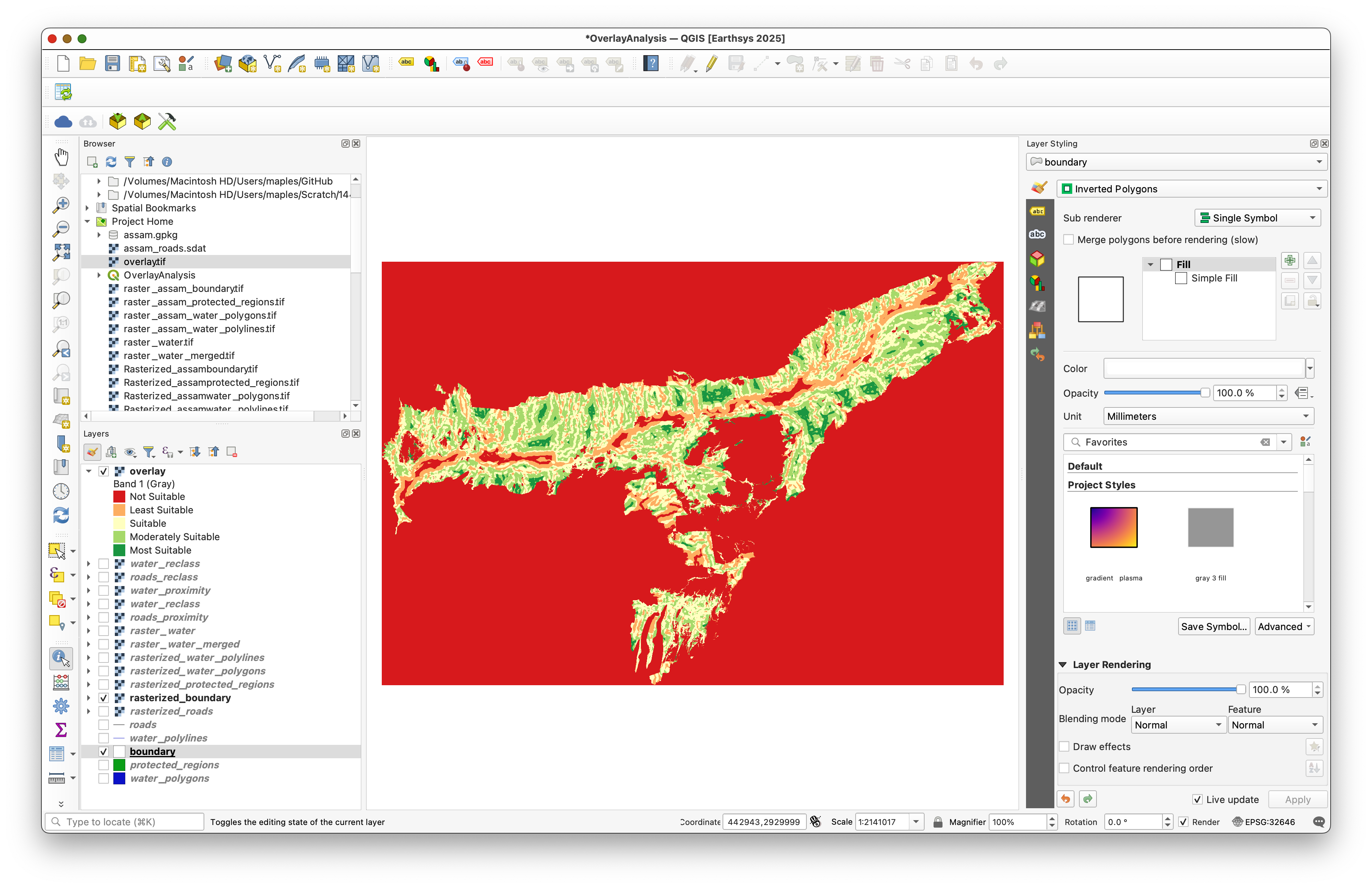
Move the boundary layer to the top of the layer stack so the masked edge appears correctly.

What You Should Turn In

If your instructor asks for a submission from this optional workshop, include:

1. The final styled overlay raster.
2. A map layout that clearly shows the suitability pattern.
3. A note describing the criteria you used and how you interpreted the result.

What This Teaches

This lab is really about workflow design.

You learned how to:

1. Convert vector layers into rasters with a shared grid.
2. Clean NoData so the layers can be combined reliably.
3. Use distance rasters to quantify proximity.
4. Reclassify rasters into scores.
5. Combine several criteria into one suitability map.

Concept Note: Raster-based overlay analysis is powerful because every criterion can be scored, weighted, and recombined. That makes it easy to update the model later if the decision rules change.